|
MATCHING WITH |
|
λ (WAVE) TRANSMISSION LINE |
|
MATCHING WITH |
|
λ (WAVE) TRANSMISSION LINE |
![]() 12 dec 2014 With PEØHZD's calculation.
12 dec 2014 With PEØHZD's calculation.
INTRODUCTION
Matching with a ¼ wave or ½ wave coaxial cable is pretty well known, but an existing 1961 system to do that with two one-twelfth-wavelength transmission lines, has not yet become common practice in many countries. This article is intended as additional attention.
SYSTEM
The system is based on a complex formula L = [arctan(sqrt (B/(B ^ 2 + B +1)))]/(2.pi), B = Z1/Z2, that can be found on the Internet together with the associated graphics. For the DIY builder the graph below is clearly enough to get started. The adjustment is quite wide-band and in principle coaxial length of one-twelfth wavelength should be sufficient, but according to the formula the matching is optimum if the length is calculated on the basis of the transformation ratio.
G3KYH's FORMULA
Leafing through my archives, I found a simple trigonometric formula derived by G3KYH, which one is able to handle well in practice. It was published, I think more than 35 years ago in Technical Topics of the English RSGB. The calculation is done in degrees and 360 should divide the outcome.
If you are like me have not "played" with trigonometry for about 50 years, you will still need to refresh your memory! Fortunately it is easy counting (after some practice) with a modern electronic pocket calculator.
Later I discovered a program on the Internet that calculates the degrees: http://leleivre.com/rf_bramham.html
But still commence some practice with the calculator.
Suppose we want to match: 75 Ohm » 50 ohms, then
cot ² ß = (75: 50) + (50 75) + 1 = 3.167,
cot √ ß = 3.167 = 1.78 (on the calculator we enter 3167 and √)
because cot ß = 1: tan ß,
thens tan ß = 1: 1 cot ß = 1.78 = 0562 (the calculator divides 1 by 1.78)
tan -1 = 29 336 ° (type 0526, shift and tan -1).
If we only focus to the calculator, see the following steps:
|
(75 : 50) + (50 : 75) + 1 = 3.167, type on the calculator 3.167 and √, = 1.78 on the calculator devide 1 by 1.78 = 0.562 type on the calculator 0.526, shift and tan -1, = 29.336° on the calculator devide 29.336 by 360, = 0.0815 |
The length of the coaxial cables is 29.336 °(degrees) that is a portion of a 360° angle.
The electrical length L of the coaxes is 29.336: 360 = 0.0815 λ (wavelength, lambda or Wave)
The physical length L is 0.0815 × W × V (velocity factor of the cables).
I rounded the numbers after the decimal point for simplicity of the example.
PEØHZD
PEØHZD made some calculations, and is write in this table.
GRAPHICS
Using the graph is simple and will satisfy in practice.
EXAMPLE 75 Ω » 50 Ω
|
If one wants transfer 75 ohms impedance to 50 ohms, that is a ratio of 75 ÷ 50 = 1.5. According to the graph it is a wavelength of 0.0814 (W)ave. The actual length of the coaxial cables dependent on the velocity factors (V) and is then: 0.0814 × W × V.
|
|
|
OK1AMF
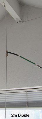
OK1AMF use this type as outdoor verticale dipole, see http://ok1amf.nagano.cz/konstrukce/Dipol144MHz/Dipol_2m.htm
EXAMPLE 100 Ω » 50 Ω
|
|
|
The transformation is 100 ÷ 50 = 2 the graph shows 0.078 wavelength.
The actual length is 0.078 × W × V.
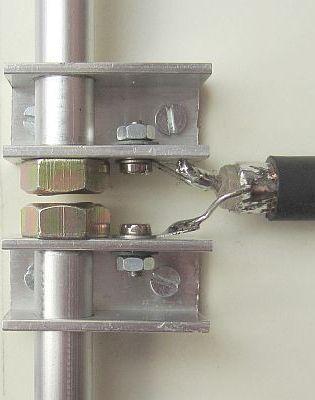
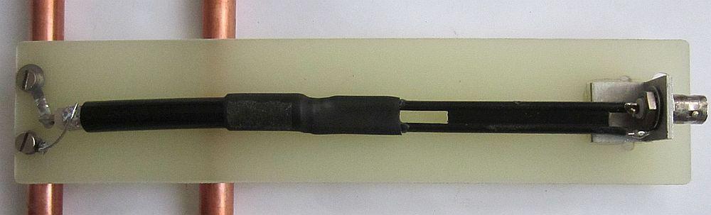
A coaxial cable of 100 ohms is obtained by connecting like («fig) the right figure e.g. two 50 Ohm cables in series. Do not forget to solder the screens together on both sides. Additional advantage is one has to deal with only one cable type.
The length of the cables has been calculated for 50.100 MHz. The table shows the SWR if an induction free 100 Ohm resistor is matched to a 50 Ohm impedance. The system is clearly broadband! The conclusion could be that one does not need too accurate calculation.

|
|
TEST ON 50 MHz
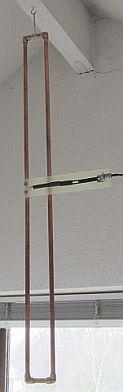
I regularly experiment in the attic with antennas including the 6 m band.
An at the ridge board («fig) hanging 6 m single loop made of insulated wire was also tested with the system. The SWR = 1.09 at 50.100 MHz is not wrong one would say in eastern part of my country. You may counter with other values because my antenna is the result of a variety of conductive materials in the vicinity and the velocity factor of the insulated wire. It's amazing what I can work in Europe with only 10 W and this antenna.
EXAMPLE 36 Ω » 50 Ω
Here we match 36 Ohm of a vertical antenna (Gp) to 50 Ohm. If we consult the graphics with the division of 50 ÷ 36 = 1.39 ohms, we find 0.0821 × W. The actual length of both coaxes is 0.0821 × W × V. A coaxial cable with impedance close to 36 Ohm (fig ») is easy to manufacture by paralleling (fig») two 75 Ohm cables.
EXAMPLE 300 Ω » 50 Ω
The figure shows that there are several options to customise. To test the system the antennas were alternately hanged at the ridge board. Recall that the results in free field can turn out differently.
![]()